Introduction to ansatz for variational quantum algorithm

This blog introduces three types of ansatz for variational quantum algorithm, including UCCSD ansatz, hardware efficient ansatz and Hamiltonian-variable ansatz.

Background

Ansatz is an important aspect of variational quantum algorithm. Generally speaking, the form of the ansatz dictates what the parameters $\theta$ are, and hence, how they can be trained to minimize the cost.[1] There are typically two types of ansatz:

• The problem-inspired ansatzes. This type of ansatz is based on the tasks at hand and can use the infomation about the problem to tailor an ansatz.
• The problem-agnostic ansatzes. This type of ansatz is not relevant to a specific problem so it can be widely adopted.

In this article, I will talk about UCCSD ansatz, Hamiltonian-variable ansatz and hardware efficient ansatz. The first and the second ones are problem-inspired ansatzes and the last is a problem-agnostic ansatz.

UCCSD ansatz

Motivation

The Unitary Coupled Cluster(UCC) ansatz is a problem-inspired ansatz widely used in quantum chemistry problems where the goal is to obtain the ground state energy of a fermionic molecular Hamiltonian $H$. The UCC ansatz proposes a candidate for such ground state based on exciting some reference state $\vert\psi_0\rangle$(usually the Hartree-Fock state of $H$). The unitary operator $e^{T - T^\dagger }$ is then applied to the reference state to get a trial state. [1]

The form of UCC ansatz is inspired by the Coupled cluster theory. Specifically, the unitary cluster operator $T - T^\dagger$ comes from the traditional coupled-cluster (TCC) and is made anti-hermitian.

General form

In UCC ansatz, the unitary operator $U$ can be expressed as [1]

where $T = \sum_i T_i$ is the fermionic excitation operator and consists of single, double, triple, . . . , up to n-fold excitations. Specifically, for UCCSD ansatz, only single and double excitations are taken into account.

In these cases, $\theta_{p}^{q}$ denotes the corresponding parameters in the ansatz. $a_i^\dagger$ denotes the fermionic creation operater at site $i$ and $a_j$ denotes the fermionic annihilation operator at site $j$.

Realization

In order to implement the ansatz on quantum device, we need to use the Trotter decomposition as individual activations don’t commute.[3]

where $t$ is the Trotter number (order of decomposition) and $T_i$ are the excitation operators. The higher order approximation could be used but it may lead to deeper circuit so it is not generally used.

Creation and annihilation operators

To fully implement the operators on the device, one need to map the operators to the native operations of a quantum computer. In the Jordan-Wigner transformation, creation and annihilation operators can be expressed by pauli operators:[3]

where $\sigma_{+,-}^k$ is the ladder operator that create/annihilation particles at site $k$. Now the question lies in how to convert exponential of strings of pauli operators to circuits, we leave the details of this part in appendix.

Pros and cons

The UCC ansatz is the first ansatz proposed for determining molecular ground states on quantum computers, which is motivated by the great success of the traditional coupled cluster theory on classical computers. However, it quickly becomes impractical for large molecules on the current noisy intermediate-scale quantum (NISQ) hardware, since the circuit depth scales as $O(N^4)$ with respect to the number of qubits $N$.[7]

Hardware efficient ansatz

Motivation

In NISQ-eradevices, short and hardware-fitting quantum circuits are preferred, to reduce the noise and get better results.

However, a unitary coupled cluster ansatz has a number of parameters that scales quartically with the number of spin orbitals that are considered in the single- and double-excitation approximation. Furthermore, as described above, the Trotterization error needs to be accounted for.[5]

Therefore, the hardware efficient ansatz comes to the rescue. It is a type of problem-agnostic ansatz that is aimed at reducing the circuit depth and the computing error.

General form

where $U^{q,i}(\theta)$ is a Euler rotation on the $q$-th qubit and at the $i$-th depth and $U_{ENT}$ are the operators in order to introduce entanglement.

Realization

Any rotation $U^{q,i}(\theta)$ can be decomposed into the form of $R_z(\theta_1)R_y(\theta_2)R_z(\theta_3)$, where $R_y = exp(iY)$.(According to the 4th chapter of ‘Quantum computing and quantum information’). After all, $R_x,R_y,R_z$ are in the set of universal quantum gates.

Besides,$U_{ENT}$ are the naturally available entangling interactions of the superconducting hardware, which are described by a drift Hamiltonian $H_0$. This Hamiltonian generates the entanglers, which are unitary operators of the form $U_{ENT}=e^{−iH_0τ}$ and entangle all the qubits in the circuit, where $\tau$ is the evolution time.

Figure: Hardware-efficient quantum circuit for trialstate preparation and energy estimation, shown here for six qubits.

Pros and cons

1. The HEA ansatz is a versatile design paradigm that can be adopted to a large number of problems. However, this also means that this ansatz doesn’t have theoretical guarantee for its performance.

2. The hardware efficient ansatz mitigates error of quantum gates because it has shallow circuit depth.

3. The hardware efficient ansatz takes into consideration the actual topological structure of the quantum bits so it saves the circuit depth overhead needed for implementing multiple-quantum gates in real laboratory conditions.

Hamiltonian-variable ansatz

Motivation

The variational Hamiltonian ansatz aims to prepare a trial ground states for a given Hamiltonian by Trotterizing an adiabatic state preparation process. It builds the variational state using rotations by terms in the Hamiltonian.[1]

This is very well suited for models such as the Hubbard model where there are few interactions terms, all of which take a simple form; in contrast, for UCC applied to the Hubbard model, the large number of possible terms will lead to a much larger circuit depth and further each term will take a more complicated form than the simple interaction in the Hubbard model.[6]

General form

The variational Hamiltonian ansatz aims to prepare a trial ground states for a given Hamiltonian. Following is its general form.

where $\theta_k$ are the variational parameters and $h_{a_k}$ are the components of the given hamiltonian $H$ such that $H = \sum_a J_a h_a$. Here $J_a$ are scalars.

Realization

With the Hubbard model, we choose the terms $a_k$ in the above equation in a repeating pattern and perform $S$ repetitions, which are called ‘steps’. In each step, there are three variational parameters, $\theta^b_h, \theta_v^b, \theta_U^b$ , where $b = 1,…,S$. Then

where $U_X(\theta)$ approximates $exp(iθ_hX)$ for $X \in {U, h, v}$ and the product is ordered by decreasing $b$. Here, ‘approximate’ is used to illustrate that the exponentials are implemented via Trotter decomposition.This Trotterization helps to approximately preserve momentum, which is useful if $\vert\Psi\rangle$ has the right momentum quantum numbers.

For $U_U, U_v$, we implement the exponential exactly. Each step of the ansatz then is a second-order Trotter approximation to evolution under $H(b) = θ_U^b h_U + θ_v^bh_v + θ_h^b h_h$.[6]

Pros and cons

Compared to UCC ansatz, the HVA ansatz uses a modest gate depth and a very modest number of variational parameters compared to the system size. In the meantime, it has theoretical guarantee on the performance. This is especially well suited for models such as the Hubbard model where there are few interactions terms, all of which take a simple form.

Appendix - How to implement exponential pauli string

To understand the exponential map of the product of Pauli spin matrices, first consider the exponential map of two $\sigma_z$ operators. To create the unitary gate $exp[−i\frac{\theta}{2} (\sigma_z \otimes \sigma_z)]$, the CNOT gate can be used to first entangle two qubits, then the $R_z$ gate is applied, and followed by a second CNOT gate.[4]

Generally, we say an operator $P$ is a Pauli string over $N$ qubits, if $P = \otimes_{j=1}^N \sigma_j^{(j)}$, where $\sigma_j \in {\mathbb{1},\sigma_x, \sigma_y, \sigma_z }$

To construct the quantum circuit corresponding to some exponential map $e^{−i \frac{\theta}{2} P}$, we use an entangling CNOT ladder between all Pauli operators $\sigma_j^{(j)} \in P$, where we choose the convention to start at the smallest $j$ and go until the largest. In the middle of this ladder, there is a $R_z(\theta)$ gate which performs a $z$-rotation by the parameter $\theta$, followed by a disentangling CNOT ladder, in reverse order as before.

Consider different pauli operators other than $\sigma^z$. We use Hardmard transformation $H$ to transform between $\sigma^x$ and $\sigma^z$ basis. We use $Rx(\frac{\pi}{2}) = exp(i\sigma^x\pi/4)$ to transform from $\sigma^z$ to $\sigma^y$ basis, and its conjugate transfer to transform in the other direction. In matrix form, \(H = \frac{1}{\sqrt{2}} \begin{bmatrix} 1 & 1\\1&-1\\ \end{bmatrix} ; Rx(\frac{\pi}{2})=\frac{1}{\sqrt{2}} \begin{bmatrix} 1 & i\\i&1\\ \end{bmatrix}\)

Below are some exemplary circuits:[3]

Exponential maps	Circuit
$e^{- i \frac{\theta}{2} \sigma_{z}^{(0)} \sigma_{z}^{(1)} \sigma_{z}^{(2)} \sigma_{z}^{(3)}}$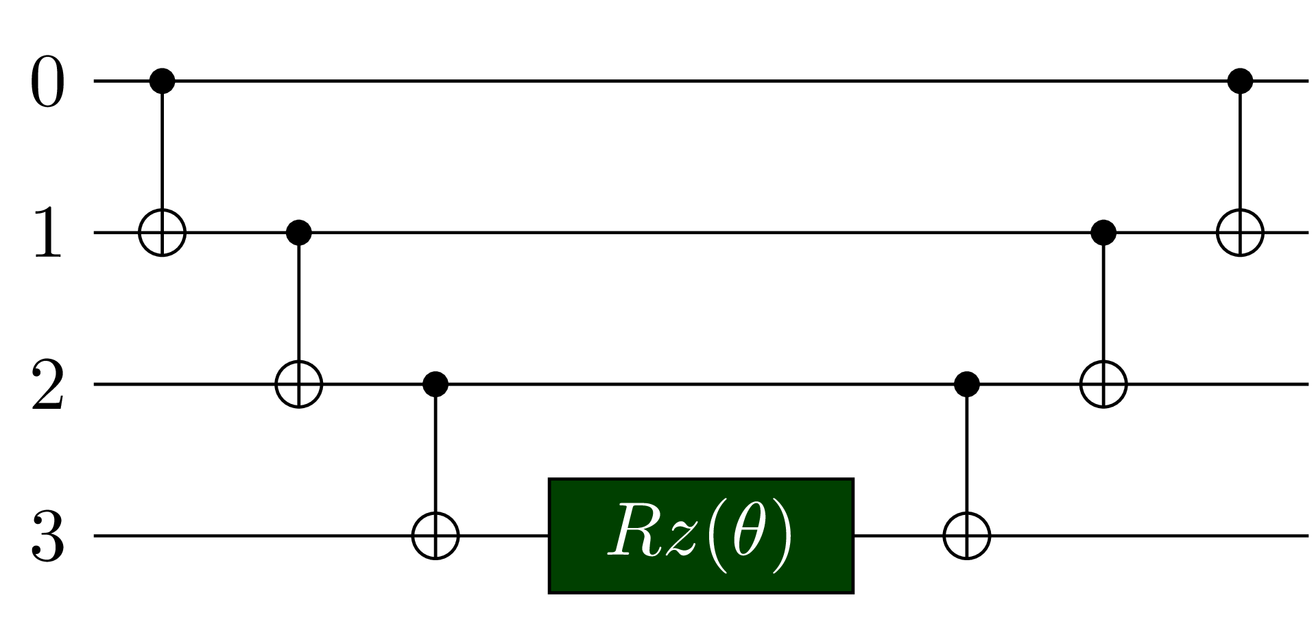
$e^{- i \frac{\theta}{2} \sigma_{x}^{(0)} \sigma_{z}^{(1)} \sigma_{z}^{(2)} \sigma_{z}^{(3)}}$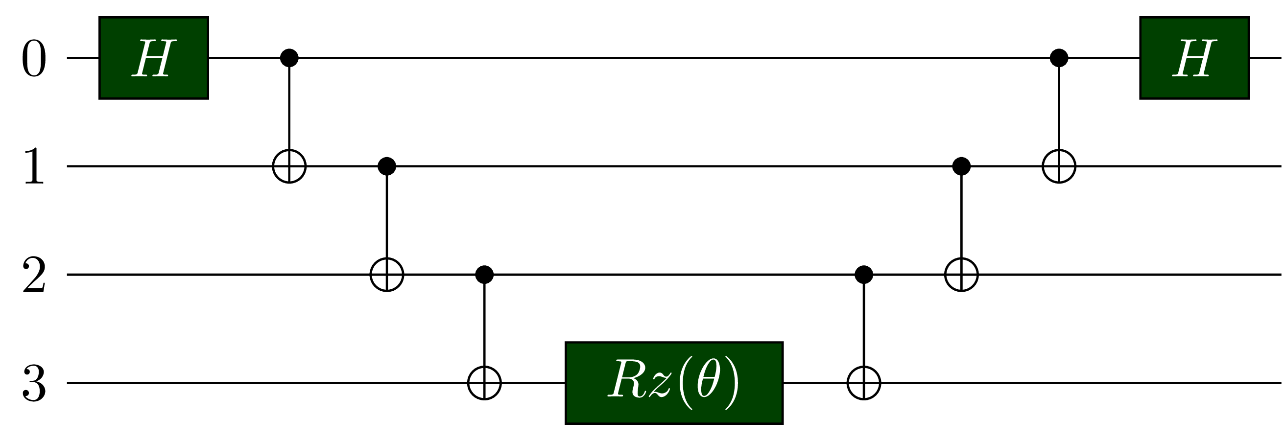
$e^{- i \frac{\theta}{2} \sigma_{y}^{(0)} \sigma_{z}^{(1)} \sigma_{z}^{(2)} \sigma_{z}^{(3)}}$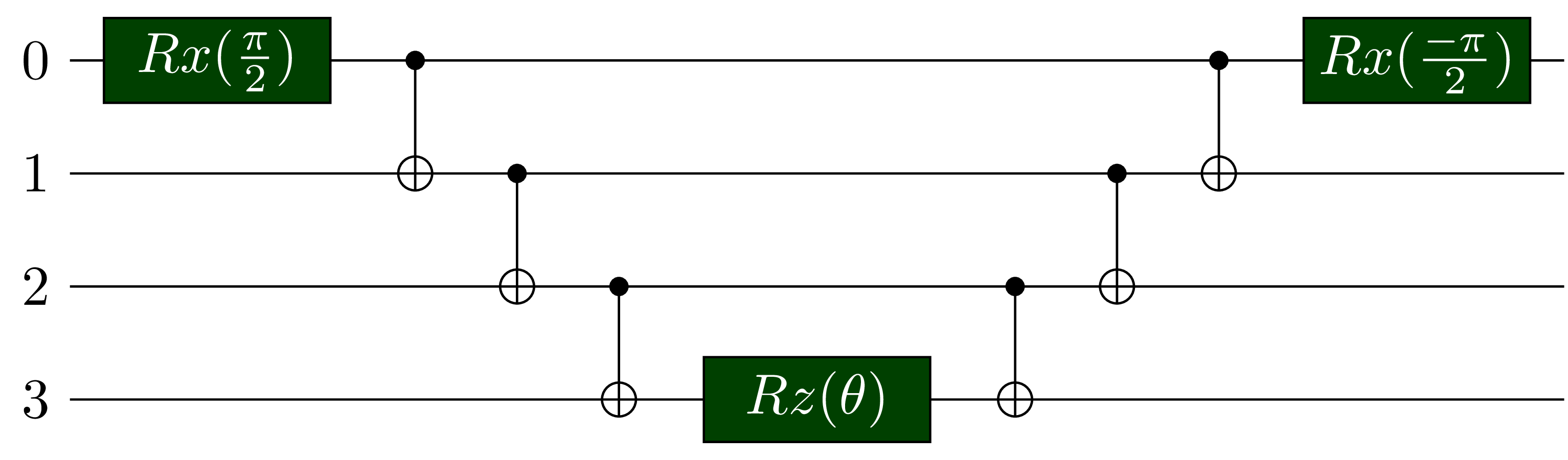
$e^{- i \frac{\theta}{2} \sigma_{x}^{(0)} \sigma_{x}^{(1)} \sigma_{y}^{(2)} \sigma_{x}^{(3)}}$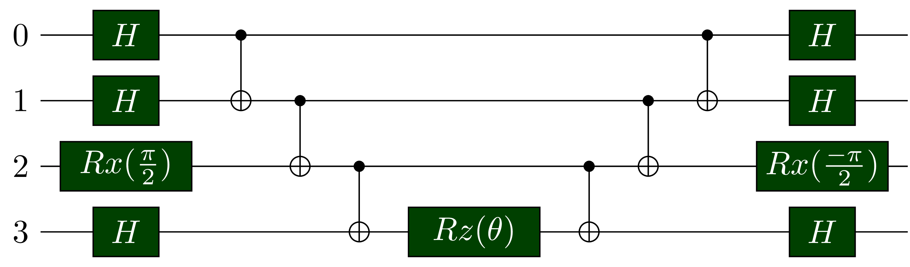

References

1. Variational quantum algorithms
2. vqas-how-do-they-work
3. A Quantum Computing View on Unitary Coupled Cluster Theory
4. Simulation of Electronic Structure Hamiltonians Using Quantum Computers
5. Hardware-efficient variational quantum eigensolver for small molecules and quantum magnets
6. Towards Practical Quantum Variational Algorithms
7. Physics-Constrained Hardware-Efficient Ansatz on Quantum Computers that is Universal, Systematically Improvable, and Size-consistent